Motion in One Dimension Definition
When we say an object is “in motion”, we mean that its position is changing with time. For one-dimensional motion, this means the object is moving only in a straight line — think of traveling straight along the x or y-axis on a graph, or a line such as \(x=2\). Or, imagine biking along a straight, flat path with no twists or turns.
Motion in one dimension is when the position of an object changes along a straight line.
 Motion in one dimension involves a change in position in only one spatial coordinate. Biking along a straight, flat path is an example of motion in one dimension, Robert Cramer via Wikimedia Commons CC BY-SA 3.0
Many quantities we use in our study of motion are vector quantities, so we need to understand the difference between vectors and scalars before continuing.
A scalar is a quantity with only magnitude and no directional value.
A vector is a quantity having both magnitude and direction.
Kinematics is the study of motion without reference to the causal forces involved. Motion in one dimension, involves situations such as traveling along a straight line or a falling object after dropping it from some height. There are a handful of variables and formulas we need to learn to understand motion in one dimension, so let’s dive into each of these next.
Motion in One Dimension Formulas
We use the following variables to describe motion in one dimension: position, displacement, distance, speed, velocity, and acceleration. You’ll want to know the meaning of each of these, as well as some important calculus-based definitions for these quantities. Let’s start with the first three variables listed.
Position, Displacement, and Distance
Knowing how to describe where an object is in space will be essential throughout your study of physics. The first variable we use to understand location is position.
The position is a vector quantity representing the spatial location of an object as measured in a defined coordinate system.
Most often, you’ll be using the two-dimensional Cartesian coordinate plane to describe both one and two-dimensional motion. To plot position, both the \(x\) and \(y\) coordinates on a 2D graph represent the object’s location in space.
 We use the two-dimensional Cartesian coordinate system to plot and analyze motion in both one and two dimensions, StudySmarter Originals
In the above graph, the initial position of some moving object is \((1,1)\) and the final position is \((3,1)\). The arrow drawn between the starting and ending positions is the displacement of the object.
Displacement is a vector quantity measuring the change in position with reference to its starting position. We calculate displacement using the following formula:
$$ \Delta x = x_f -x_0, $$
where \(x\) is the position variable and \(x_0\) is the initial position.
The \(\Delta x\) is read out loud as “the change in x” or “delta x”. In our example graph above, the displacement is \(\Delta x = (3-1) = 2\) units of length. So, if the units of length were meters, the total displacement of the moving object is \(2\) meters. You might be wondering, how does this relate to the distance traveled — aren’t they the same? The answer is no!
Distance is a scalar quantity measuring the total length traveled with reference to the starting position.
We measure both displacement and distance in units of length, most commonly meters, or \(\mathrm{m}\). The direction of travel is very critical for displacement, so pay attention as you calculate! The displacement of an object can be zero if we end at the same place we started, but the total distance will always be nonzero if we’ve moved at all. In our graph, the distance traveled is the same as the displacement here. However, if the object traveled back to its initial position, then the displacement would be zero with a total distance traveled of \(4\) units.
Speed and Velocity
The next two quantities we use for motion in one dimension are speed and velocity.
Speed is a scalar quantity measuring the change in distance over a time interval. Mathematically, we define speed as:
$$ s=\frac{d}{t}, $$
where \(d\) is the total distance traveled and \(t\) is the elapsed time.
Similar to the difference between distance and displacement, the key distinction between speed and velocity is that velocity is a vector quantity, while speed is not.
Velocity is a vector quantity measuring the rate of displacement change over the change in time. Mathematically, we define velocity in the x-direction as:
$$ v_x = \frac{\mathrm{d}}{\mathrm{d}t}\left(x\left(t\right)\right), $$
the first derivative of the position function with respect to time.
We measure both speed and velocity in units of length per time, most commonly meters per second, or \(\frac{\mathrm{m}}{\mathrm{s}}\). Differentiating the rate of change in position of a moving object with respect to time will give us the instantaneous velocity, or the velocity measured at a specific moment in time:
$$ v_{x\,(\mathrm{inst})} = \frac{\mathrm{d}x}{\mathrm{d}t}. $$
If instead, we want to find the average velocity, we can use the following formula:
$$ v_{x\,(\mathrm{avg})} = \frac{x_f-x_0}{t_f-t_0} = \frac{\Delta x}{\Delta t}, $$
where \(\Delta x\) is the change in position and \(\Delta t\) is the change in time. This formula is useful if you’re given the numerical values of the starting and ending positions and time.
Another way of writing the mathematical formula for velocity is:
\begin{align*} v\left(t\right) &= \ x'\left(t\right) \\ x\left(t\right) &= \int{v(t)\mathrm{d}t} \end{align*}
In words, this means the first derivative of an object’s position function gives the velocity function, and the integral of the velocity function gives the position function. These operations are both taken with respect to time. You’ll use these relationships to determine one function given the other.
Acceleration
We define the acceleration of an object undergoing motion in one dimension as follows.
Acceleration is a vector quantity measuring the rate of velocity change over time. Mathematically, we define acceleration as:
\begin{align*} a_x &= \frac{\mathrm{d}}{\mathrm{d}t}v_x(t) \\ &= \frac{\mathrm{d}^2}{\mathrm{d}t^2}x(t), \end{align*}
the first derivative of the velocity function with respect to time, and the second derivative of the position function with respect to time.
We measure acceleration in units of length per squared unit of time, most commonly meters per second squared, or \(\frac{\mathrm{m}}{\mathrm{s}^2}\). Put simply, acceleration is changing velocity. This velocity change can be either speeding up or slowing down, or a directional change as well. The instantaneous acceleration, or acceleration at a specific moment in time, is:
$$ a_{x\,(\mathrm{inst})} = \frac{\mathrm{d}v}{\mathrm{d}t}. $$
To find the average acceleration over a period of time, we use the formula:
$$ a_{x\,(\mathrm{avg})} = \frac{v_f-v_0}{t_f-t_0} = \frac{\Delta v}{\Delta t}, $$
where \(\Delta v\) is the change in velocity. Finally, we can again write this relationship between position, velocity, and acceleration functions differently using calculus:
\begin{align*} a(t) &= v'(t) = x''(t) \\ v(t) &= \int{a(t)\mathrm{d}t} \\ x(t) &= \int{v(t)\mathrm{d}t} = \iint{a(t)\mathrm{d}t}. \end{align*}
In words, this says that the velocity function is the integral of the acceleration function, and the position function is the double integral of the acceleration function.
Describing Motion and Kinematics in One Dimension
Aside from the variables we just introduced, one of the most important tools for describing one-dimensional motion and kinematics are graphs. A few of the plots you’ll need to understand both how to interpret and create are:
Position-time graphs, showing the distance traveled over time from the starting point.
Velocity-time graphs, showing the changes in velocity over time.
Acceleration-time graphs, showing the changes in acceleration over time.
Let’s take a brief look at each of these three types of graphs.
A position-time graph plots the position \(x\) along the vertical axis and the time \(t\) along the horizontal axis.
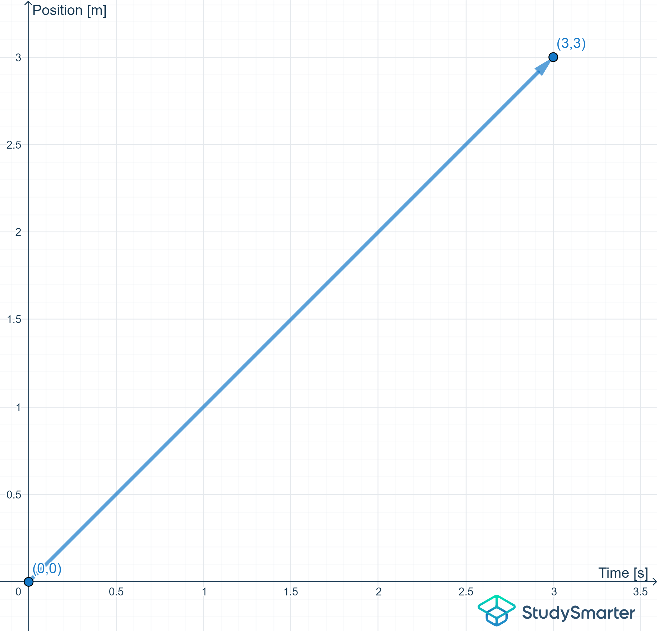
Plotting the position against time gives us the distance traveled. We can also determine the velocity by finding the slope of the curve, StudySmarter Originals
In this plot, the magnitude of the position vector will give us the distance traveled:
$$ \Delta x = 3-0 = 3\,\mathrm{m}. $$
The slope of a position-time graph at a given point will give us the velocity value at that point. When the slope is zero, the velocity will also be zero. The slope of this line is simply equal to \(1\), so the velocity here is \(1\,\frac{\mathrm{m}}{\mathrm{s}}\).
Next, let’s look at a velocity-time graph.
A velocity-time graph plots the velocity along the vertical axis and the time along the horizontal axis.
 Plotting the velocity against time shows the increases and decreases in velocity. We can also determine the acceleration at any point by finding the slope of a tangent line at that point, StudySmarter Originals
The area under velocity-time graphs will give the displacement of the moving object. In this graph, if we calculate the area in the yellow-shaded rectangle, we will find the displacement that occurred between times \(t_1\) and \(t_2\). Finding the slope of a point along the curve gives us the acceleration at that moment in time.
Now, what is happening to the acceleration before, during, and after time \(t_1\)? In the plot above, there are three tangent lines near the region of max velocity. These straight lines have an equivalent slope to the curve at that point. Just before time \(t_1\), the slope of the tangent line is negative, indicating a deceleration of the object and therefore decreasing velocity.
Finally, let’s examine an acceleration-time graph.
An acceleration-time graph plots the acceleration along the vertical axis and the time along the horizontal axis.
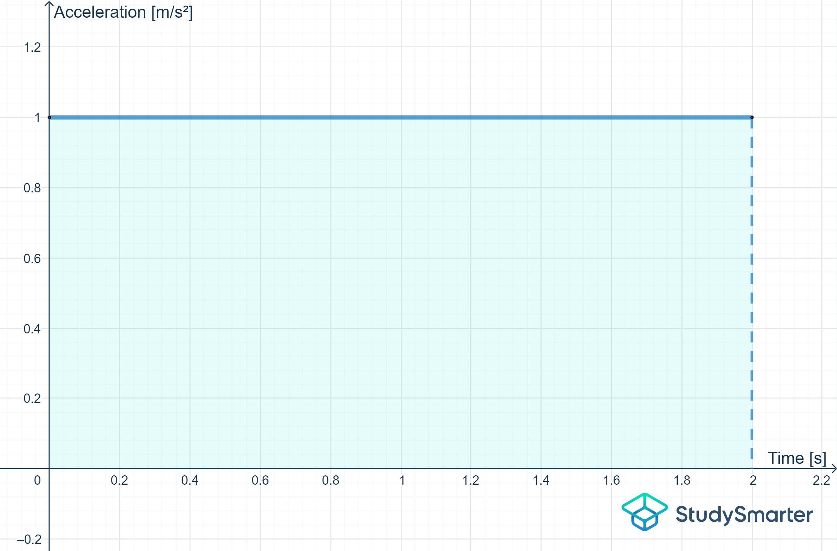
Acceleration plotted against time shows if the acceleration is changing or constant. The area under the curve represents the change in velocity, StudySmarter Originals
The area under acceleration-time graphs will give the change in velocity \(\Delta v\) of a moving object during the time interval covered on the plot. In this graph, the moving object in question has a constant acceleration of \(1\,\frac{\mathrm{m}}{\mathrm{s}^2}\). For now, you likely won’t use these graphs as much, but it’s still beneficial to know what to expect.
You might be wondering what we’re measuring with acceleration-time graphs. The rate of change of acceleration is another motion variable called jerk. Jerk is defined mathematically as:
$$ \mathrm{jerk} = \frac{\Delta a}{\Delta t}, $$
where \(\Delta a\) is the change in acceleration. On an acceleration-time graph, the slope of the curve gives the value of the jerk at a specific point in time. If the name of this variable sounds odd, think of it as the jerky type of motion that happens when you suddenly change your acceleration, such as slamming on the brakes in a moving car.
Graphs of motion in one dimension, along with some calculus, are powerful aids for understanding all sorts of motion. Now that we’ve walked through the tools we need, let’s look at a common problem type: vertical projectile motion in one dimension.
Vertical Projectile Motion in One Dimension
One of the first types of problems you’ll encounter is projectile motion.
Projectile motion is the motion of an object that is thrown into the air, accelerating only due to gravity.
Vertical projectile motion is the motion of a thrown object upwards, having only a vertical component to its velocity.
 An object thrown directly up in the air will accelerate downwards due to gravity, MikeRun via Wikimedia Commons CC BY-SA 4.0
In a vertical projectile motion problem, we throw an object like a ball up in the air, starting at an initial vertical position of \(h_0\). While tossing, we only give the object an initial vertical velocity \(v_{x,0}\); the horizontal component is zero. After the initial throw, the ball reaches a maximum height before accelerating back downwards due to gravity. This is just a brief introduction — we’ll go into the specifics of vertical projectile motion in one dimension later on.
Motion in One Dimension Examples
To finish our introduction to motion in one dimension, let’s walk through an example
An object travels with the velocity function \(v(t) = 5.5\frac{\mathrm{m}}{\mathrm{s}^2} \cdot t+2\,\frac{\mathrm{m}}{\mathrm{s}} \). What distance does the object travel in half a minute?
We’ll use the most common units for velocity and measure in standard units of \(\frac{\mathrm{m}}{\mathrm{s}}. Recall the relationship between position and velocity:
$$ x(t) = \int v(t) \mathrm{d}t. $$
We want to integrate the velocity function over the time interval, starting from zero and ending at \(30\) seconds.
\begin{align*} x(t) &= \int_0^{30} \left(5.5\frac{\mathrm{m}}{\mathrm{s}^2} \cdot t+2\,\frac{\mathrm{m}}{\mathrm{s}}\right)\mathrm{d}t \\ x(t) &= \frac{5.5\frac{\mathrm{m}}{\mathrm{s}^2} \cdot t^2}{2} + 2\,\frac{\mathrm{m}}{\mathrm{s}}\cdot t \\ x(30\,\mathrm{s}) &= \frac{5.5\frac{\mathrm{m}}{\mathrm{s}^2} \cdot (30\,\mathrm{s})^2}{2} + 2\,\frac{\mathrm{m}}{\mathrm{s}}\cdot 30\,\mathrm{s} \\ x(30\,\mathrm{s}) &= 2475\,\mathrm{m} + 60\,\mathrm{m} \\ x(30\,\mathrm{s}) &= 2535\,\mathrm{m}\end{align*}
The object travels \(2535\,\mathrm{m}\) over \(30\,\mathrm{s}\).
Let’s walk through one more example, this time using the calculus definition of velocity.
An object moves along the x-axis with a position equation of \(x(t) = 4\frac{\mathrm{m}}{\mathrm{s}^2}\cdot t^2-7\frac{\mathrm{m}}{\mathrm{s}} \cdot t+3\mathrm{m}\), with \(x\) measured in \(m)\). At time \(t=5\,\mathrm{s}\), what is the instantaneous velocity of the object?
We know that the relationship between the velocity and position of an object undergoing one-dimensional motion is:
$$ v(t) = x'(t). $$
First, we want to take the second derivative of the position function given above.
\begin{align*} v(t) &= x'(t) \\ v(t) &= \frac{\mathrm{d}}{\mathrm{d}t}\left(4\frac{\mathrm{m}}{\mathrm{s}^2}\cdot t^2-7\frac{\mathrm{m}}{\mathrm{s}} \cdot t+3\mathrm{m} \right) \\ v(t) &= 8\,\frac{\mathrm{m}}{\mathrm{s}^2} \cdot t-7\,\frac{\mathrm{m}}{\mathrm{s}}. \end{align*}
Finally, we plug in our value of \(t\) and solve for the velocity:
\begin{align*} v(5\,\mathrm{s}) &= 8\,\frac{\mathrm{m}}{\mathrm{s}^2} \cdot (5\,\mathrm{s})-7\,\frac{\mathrm{m}}{\mathrm{s}} \\ v(5\,\mathrm{s}) &= 33\,\frac{\mathrm{m}}{\mathrm{s}}.\end{align*}
At \(t=5\,\mathrm{s}\), the object’s velocity is equal to \(33\,\frac{\mathrm{m}}{\mathrm{s}}.
Now that you’ve seen an introduction to motion in one dimension, your next step is to learn one-dimensional kinematics, or the study of motion without reference to the forces involved. We’ll be going into more kinematics formulas for motion in one dimension in the Kinematics Equations article, so read on!
Motion in One Dimension - Key takeaways
- Motion in one dimension is the change in position of an object along a single spatial dimension.
- We can identify if an object is in motion by examining its position and direction changes, or velocity, along a path.
- Position is the vector quantity measuring the spatial location of an object, most often represented with a pair of coordinates.
- Displacement is the vector quantity measuring the change in position of an object with respect to its initial position, calculated using the formula \(\Delta x = x_f-x_0\).
- Distance is the scalar quantity measuring the total length an object travels over a measured period of time.
- Speed is the scalar quantity measuring the distance traveled over a period of time and describes how fast an object traveled without respect to direction, calculated using the formula \(s=\frac{d}{t}\).
- Velocity is the vector quantity measuring the rate of change of position with respect to time, or \(v_x = \frac{\mathrm{d}x}{\mathrm{d}t}\).
- Acceleration is the vector quantity measuring the rate of change of velocity with respect to time, or \(a_x = \frac{\mathrm{d}v}{\mathrm{d}t}\).
Similar topics in Physics
Related topics to Kinematics Physics


