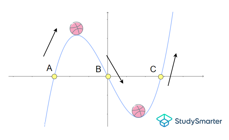
The trajectory of a ball example
The ball begins its journey from point A where it goes uphill. It then reaches the peak of the hill and rolls down to point B where it meets a trench. At the foot of the trench, the ball finally continues uphill again to point C.
Now, observe the curve made by the movement of this ball. Doesn't it remind you of a cubic function graph? That's right, it is! In this lesson, you will be introduced to cubic functions and methods in which we can graph them.
Definition of a Cubic Function
To begin, we shall look into the definition of a cubic function.
A cubic function is a polynomial function of degree three. In other words, the highest power of \(x\) is \(x^3\).
The standard form is written as
\[f(x)=ax^3+bx^2+cx+d,\]
where \(a,\ b,\ c\) and \(d\) are constants and \(a ≠ 0\).
Here are a few examples of cubic functions.
Examples of cubic functions are
\[f(x)=x^3-2,\]
\[g(x)=-2x^3+3x^2-4x,\]
\[h(x)=\frac{1}{2}x^3+4x-1.\]
Notice how all of these functions have \(x^3\) as their highest power.
Like many other functions you may have studied so far, a cubic function also deserves its own graph.
Prior to this topic, you have seen graphs of quadratic functions. Recall that these are functions of degree two (i.e. the highest power of \(x\) is \(x^2\)). We learnt that such functions create a bell-shaped curve called a parabola and produce at least two roots.
So what about the cubic graph? In the following section, we will compare cubic graphs to quadratic graphs.
Cubic Graphs vs. Quadratic Graphs Characteristics
Before we compare these graphs, it is important to establish the following definitions.
The axis of symmetry of a parabola (curve) is a vertical line that divides the parabola into two congruent (identical) halves.
The point of symmetry of a parabola is called the central point at which
- the curve divides into two equal parts (that are of equal distance from the central point);
- both parts face different directions.
The table below illustrates the differences between the cubic graph and the quadratic graph.
Property | Quadratic Graph | Cubic Graph |
Basic Equation | \[y=x^2\] | \[y=x^3\] |
Basic Graph | 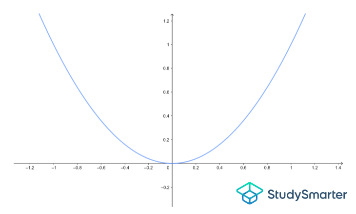
Basic quadratic function graph The axis of symmetry is about the origin (0,0) | 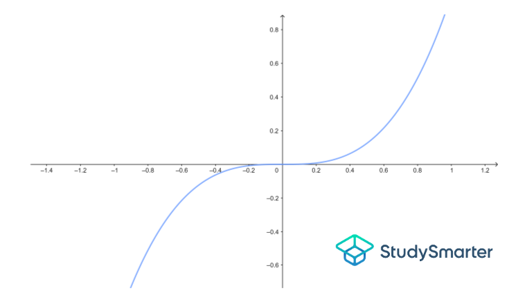
Basic cubic function graph The point of symmetry is about the origin (0,0) |
Number of Roots(By Fundamental Theorem of Algebra) | 2 solutions | 3 solutions |
Domain | Set of all real numbers | Set of all real numbers |
Range | Set of all real numbers | Set of all real numbers |
Type of Function | Even | Odd |
Axis of Symmetry | Present | Absent |
Point of Symmetry | Absent | Present |
Turning Points | One: can either be a maximum or minimum value, depending on the coefficient of \(x^2\) | Zero: this indicates that the root has a multiplicity of three (the basic cubic graph has no turning points since the root x = 0 has a multiplicity of three, x3 = 0) |
OR |
Two: this indicates that the curve has exactly one minimum value and one maximum value |
Graphing Cubic Functions
We will now be introduced to graphing cubic functions. There are three methods to consider when sketching such functions, namely
Transformation;
Factorisation;
Constructing a Table of Values.
With that in mind, let us look into each technique in detail.
Cubic function graph transformation
In Geometry, a transformation is a term used to describe a change in shape. Likewise, this concept can be applied in graph plotting. By altering the coefficients or constants for a given cubic function, you can vary the shape of the curve.
Let's return to our basic cubic function graph, \(y=x^3\).
Basic cubic polynomial graph
There are three ways in which we can transform this graph. This is described in the table below.
Form of Cubic Polynomial | Change in Value | Variations | Plot of Graph |
\[y=\mathbf{a}x^3\] | Varying \(a\) changes the cubic function in the y-direction, i.e. the coefficient of \(x^3\) affects the vertical stretching of the graph | In doing so, the graph gets closer to the y-axis and the steepness raises. If \(a\) is small (0 < \(a\) < 1), the graph becomes flatter (orange) If \(a\) is negative, the graph becomes inverted (pink curve)
| 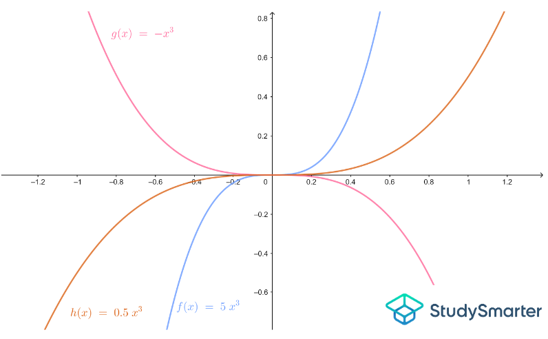
Transformation: change of coefficient a |
\[y=x^3+\mathbf{k}\] | Varying \(k\) shifts the cubic function up or down the y-axis by \(k\) units | If \(k\) is negative, the graph moves down \(k\) units in the y-axis (blue curve) If \(k\) is positive, the graph moves up \(k\) units in the y-axis (pink curve)
| 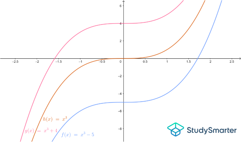
Transformation: change of constant k |
\[y=(x-\mathbf{h})^3\] | Varying \(h\) changes the cubic function along the x-axis by \(h\) units. | If \(h\) is negative, the graph shifts \(h\) units to the left of the x-axis (blue curve) If \(h\) is positive, the graph shifts \(h\) units to the right of the x-axis (pink curve)
| 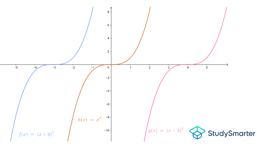
Transformation: change of constant h |
Let us now use this table as a key to solve the following problems.
Plot the graph of
\[y=–4x^3–3.\]
Solution
Step 1: The coefficient of \(x^3\) is negative and has a factor of 4. Thus, we expect the basic cubic function to be inverted and steeper compared to the initial sketch.

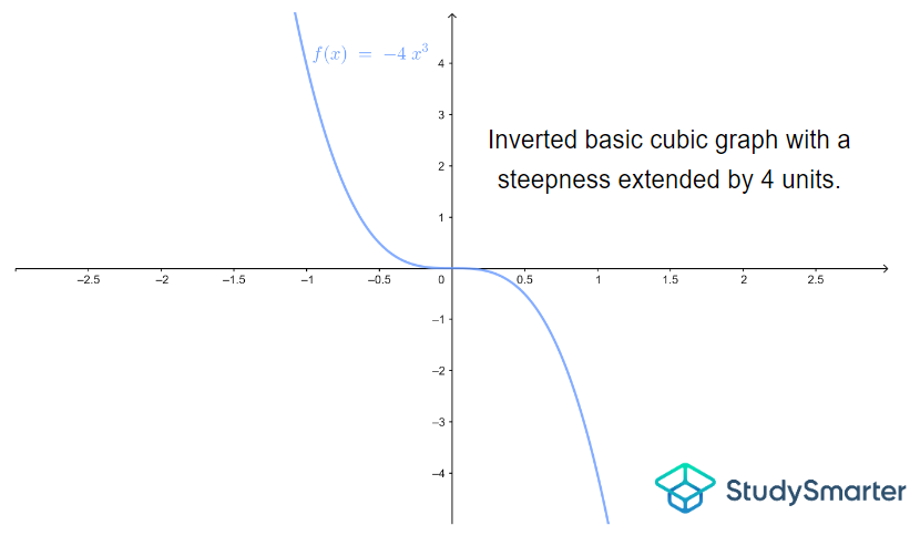
Step 1, Example 1
Step 2: The term –3 indicates that the graph must move 5 units down the \(y\)-axis. Thus, taking our sketch from Step 1, we obtain the graph of \(y=–4x^3–3\) as:
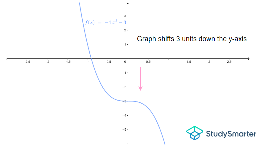
Step 2, Example 1
Here is another worked example.
Plot the graph of
\[y=(x+5)^3+6.\]
Solution
Step 1: The term \((x+5)^3\) indicates that the basic cubic graph shifts 5 units to the left of the x-axis.
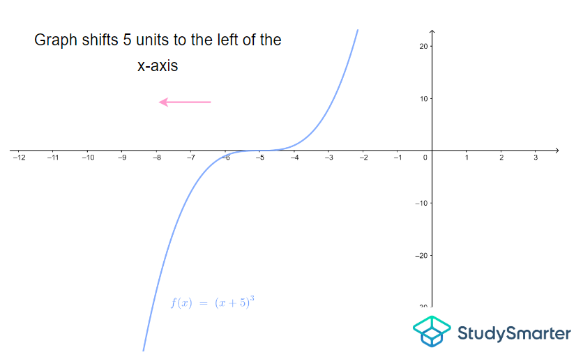
Step 1, Example 2
Step 2: Finally, the term +6 tells us that the graph must move 6 units up the y-axis. Hence, taking our sketch from Step 1, we obtain the graph of \(y=(x+5)^3+6\) as:
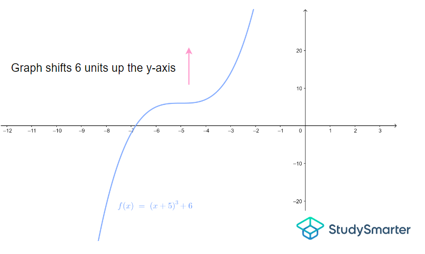
Step 2, Example 2
Vertex Form of Cubic Functions
From these transformations, we can generalise the change of coefficients \(a, k\) and \(h\) by the cubic polynomial
\[y=a(x–h)^3+k.\]
This is known as the vertex form of cubic functions. Recall that this looks similar to the vertex form of quadratic functions. Notice that varying \(a, k\) and \(h\) follow the same concept in this case. The only difference here is that the power of \((x – h)\) is 3 rather than 2!
Factorisation
In Algebra, factorising is a technique used to simplify lengthy expressions. We can adopt the same idea of graphing cubic functions.
There are four steps to consider for this method.
Step 1: Factorise the given cubic function.
If the equation is in the form \(y=(x–a)(x–b)(x–c)\), we can proceed to the next step.
Step 2: Identify the \(x\)-intercepts by setting \(y=0\).
Step 3: Identify the \(y\)-intercept by setting \(x=0\).
Step 4: Plot the points and sketch the curve.
Here is a worked example demonstrating this approach.
Factorising takes a lot of practice. There are several ways we can factorise given cubic functions just by noticing certain patterns. To ease yourself into such a practice, let us go through several exercises.
Plot the graph of
\[y=(x+2)(x+1)(x-3).\]
Solution
Observe that the given function has been factorised completely. Thus, we can skip Step 1.
Step 2: Find the x-intercepts
Setting \(y=0\), we obtain \((x+2)(x+1)(x-3)=0\).
Solving this, we obtain three roots, namely
\[x=–2,\ x=-1,\ x=3\]
Step 3: Find the y-intercept
Plugging \(x=0\), we obtain
\[y=(0+2)(0+1)(0-3)=(2)(1)(-3)=-6\]
Thus, the y-intercept is \(y=-6\).
Step 4: Sketch the graph
As we have now identified the \(x\) and \(y\)-intercepts, we can plot this on the graph and draw a curve to join these points together.
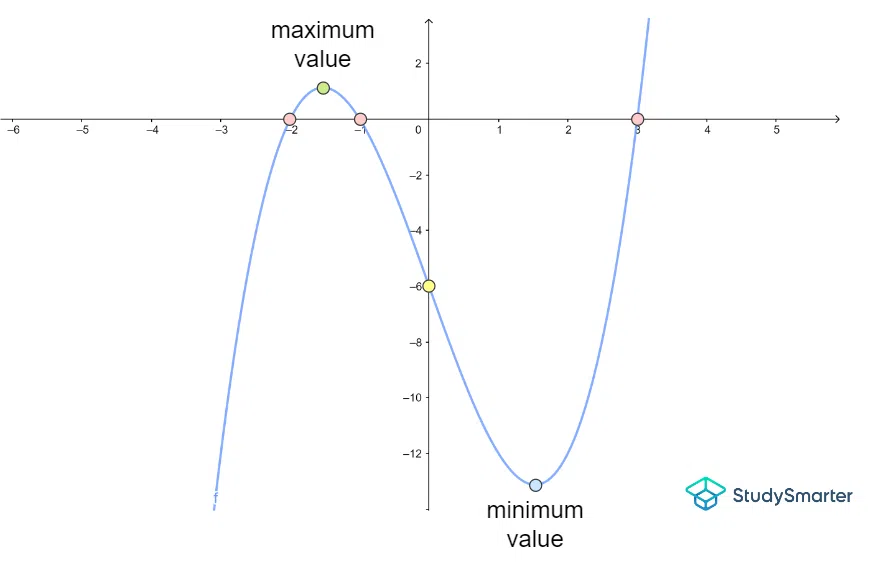
Graph for Example 3
The pink points represent the \(x\)-intercepts.
The yellow point represents the \(y\)-intercept.
Notice that we obtain two turning points for this graph:
- a maximum value between the roots \(x=–2\) and \(x=1\). This is indicated by the green point.
- a minimum value between the roots \(x=1\) and \(x=3\). This is indicated by the blue point.
The maximum value is the highest value of \(y\) that the graph takes. The minimum value is the smallest value of \(y\) that the graph takes.
Let's take a look at another example.
Plot the graph of
\[y=(x+4)(x^2–2x+1).\]
Solution
Step 1: Notice that the term \(x^2–2x+1\) can be further factorized into a square of a binomial. We can use the formula below to factorize quadratic equations of this nature.
A binomial is a polynomial with two terms.
The Square of a Binomial
\[(a-b)^2=a^2-2ab+b^2\]
Using the formula above, we obtain \((x–1)^2\).
Thus, the given cubic polynomial becomes
\[y=(x+4)(x–1)^2\]
Step 2: Setting \(y=0\), we obtain
\[(x+4)(x–1)^2=0\]
Solving this, we have the single root \(x=–4\) and the repeated root \(x=1\).
Note here that \(x=1\) has a multiplicity of 2.
Step 3: Plugging \(x=0\), we obtain
\[y=(0+4)(0–1)^2=(4)(1)=4\]
Thus, the y-intercept is \(y=4\).
Step 4: Plotting these points and joining the curve, we obtain the following graph.
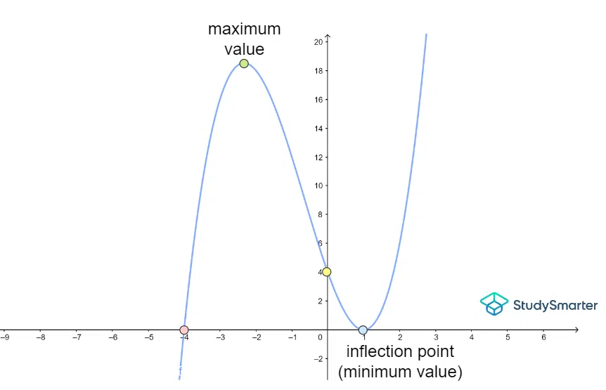
Graph for Example 4
The pink points represent the \(x\)-intercept.
The blue point is the other \(x\)-intercept, which is also the inflection point (refer below for further clarification).
The yellow point represents the \(y\)-intercept.
Again, we obtain two turning points for this graph:
- a maximum value between the roots \(x=–4\) and \(x=1\). This is indicated by the green point.
- a minimum value at \(x=1\). This is indicated by the blue point.
For this case, since we have a repeated root at \(x=1\), the minimum value is known as an inflection point. Notice that from the left of \(x=1\), the graph is moving downwards, indicating a negative slope whilst from the right of \(x=1\), the graph is moving upwards, indicating a positive slope.
An inflection point is a point on the curve where it changes from sloping up to down or sloping down to up.
Constructing a Table of Values
Before we begin this method of graphing, we shall introduce The Location Principle.
The Location Principle
Suppose \(y = f(x)\) represents a polynomial function. Let \(a\) and \(b\) be two numbers in the domain of \(f\) such that \(f(a) < 0\) and \(f(b) > 0\). Then the function has at least one real zero between \(a\) and \(b\).
The Location Principle will help us determine the roots of a given cubic function since we are not explicitly factorising the expression. For this technique, we shall make use of the following steps.
Step 1: Evaluate \(f(x)\) for a domain of \(x\) values and construct a table of values (we will only consider integer values);
Step 2: Locate the zeros of the function;
Step 3: Identify the maximum and minimum points;
Step 4: Plot the points and sketch the curve.
This method of graphing can be somewhat tedious as we need to evaluate the function for several values of \(x\). However, this technique may be helpful in estimating the behaviour of the graph at certain intervals.
Note that in this method, there is no need for us to completely solve the cubic polynomial. We are simply graphing the expression using the table of values constructed. The trick here is to calculate several points from a given cubic function and plot it on a graph which we will then connect together to form a smooth, continuous curve.
Graph the cubic function
\[f(x)=2x^3+5x^2-1.\]
Solution
Step 1: Let us evaluate this function between the domain \(x=–3\) and \(x=2\). Constructing the table of values, we obtain the following range of values for \(f(x)\).
| \(x\) | \(f(x)\) |
| –3 | –10 |
| –2 | 3 |
| -1 | 2 |
| 0 | -1 |
| 1 | 6 |
| 2 | 35 |
Step 2: Notice that between \(x=-3\) and \(x=-2\) the value of \(f(x)\) changes sign. The same change in sign occurs between \(x=-1\) and \(x=0\). And again in between \(x=0\) and \(x=1\).
The Location Principle indicates that there is a zero between these two pairs of \(x\)-values.
Step 3: We first observe the interval between \(x=-3\) and \(x=-1\). The value of \(f(x)\) at \(x=-2\) seems to be greater compared to its neighbouring points. This indicates that we have a relative maximum.
Similarly, notice that the interval between \(x=-1\) and \(x=1\) contains a relative minimum since the value of \(f(x)\) at \(x=0\) is lesser than its surrounding points.
We use the term relative maximum or minimum here as we are only guessing the location of the maximum or minimum point given our table of values.
Step 4: Now that we have these values and we have concluded the behaviour of the function between this domain of \(x\), we can sketch the graph as shown below.
Graph for Example 5
The pink points represent the \(x\)-intercepts.
The green point represents the maximum value.
The blue point represents the minimum value.
Examples of Cubic Function Graphs
In this final section, let us go through a few more worked examples involving the components we have learnt throughout cubic function graphs.
Plot the graph of
\[y=x^3-7x-6\]
given that \(x=–1\) is a solution to this cubic polynomial.
Solution
Step 1: By the Factor Theorem, if \(x=-1\) is a solution to this equation, then \((x+1)\) must be a factor. Thus, we can rewrite the function as
\[y=(x+1) (ax^2+bx+c)\]
Note that in most cases, we may not be given any solutions to a given cubic polynomial. Hence, we need to conduct trial and error to find a value of \(x\) where the remainder is zero upon solving for \(y\). Common values of \(x\) to try are 1, –1, 2, –2, 3 and –3.
To find the coefficients \(a\), \(b\) and \(c\) in the quadratic equation \(ax^2+bx+c\), we must conduct synthetic division as shown below.
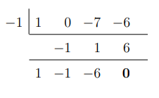
Synthetic division for Example 6
By looking at the first three numbers in the last row, we obtain the coefficients of the quadratic equation and thus, our given cubic polynomial becomes
\[y=(x+1)(x^2–x–6)\]
We can further factorize the expression \(x^2–x–6\) as \((x–3)(x+2)\).
Thus, the complete factorized form of this function is
\[y=(x+1)(x–3)(x+2)\]
Step 2: Setting \(y=0\), we obtain
\[(x+1)(x–3)(x+2)=0\]
Solving this, we obtain three roots:
\[x=–2,\ x=–1,\ x=3\]
Step 3: Plugging \(x=0\), we obtain
\[y = (0 + 1) (0 – 3) (0 + 2) = (1) (–3) (2) = –6\]
Thus, the y-intercept is \(y = –6\).
Step 4: The graph for this given cubic polynomial is sketched below.
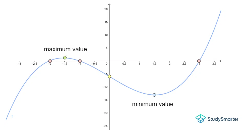
Graph for Example 6
The pink points represent the \(x\)-intercepts.
The yellow point represents the \(y\)-intercept.
Once more, we obtain two turning points for this graph:
- a maximum value between the roots \(x = –2\) and \(x = –1\). This is indicated by the green point.
- a minimum value between the roots \(x = –1\) and \(x = 3\). This is indicated by the blue point.
Here is our final example for this discussion.
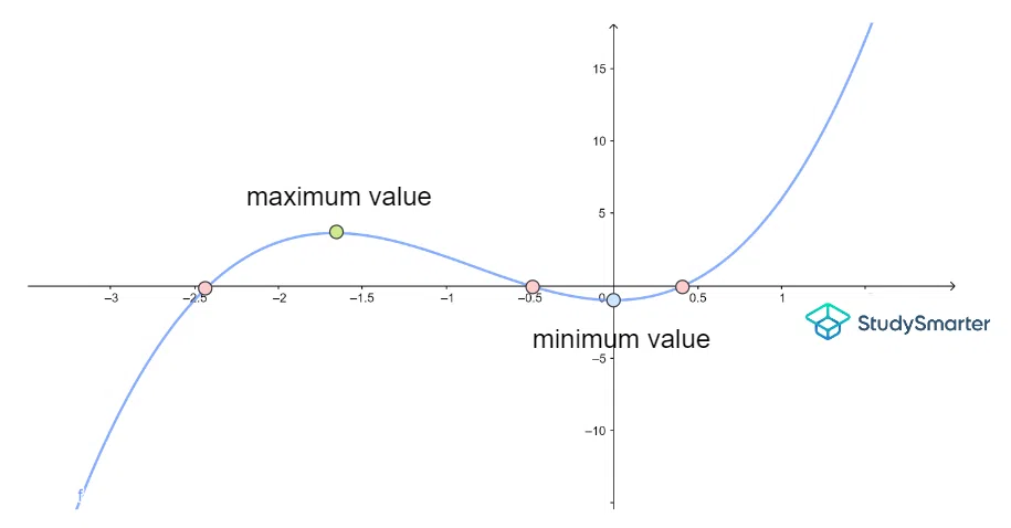
Plot the graph of
\[y=-(2x–1)(x^2–1).\]
Solution
Firstly, notice that there is a negative sign before the equation above. This means that the graph will take the shape of an inverted (standard) cubic polynomial graph. In other words, this curve will first open up and then open down.
Step 1: We first notice that the binomial \((x^2–1)\) is an example of a perfect square binomial.
We can use the formula below to factorise quadratic equations of this nature.
The Perfect Square Binomial
\[(a^2-b^2)^2=(a+b)(a-b)\]
Using the formula above, we obtain \((x+1)(x-1)\).
Thus, the complete factored form of this equation is
\[y = – (2x – 1)(x + 1) (x – 1)\]
Step 2: Setting \(y=0\), we obtain
\[(2x-1)(x+1)(x-1)=0\]
Solving this, we obtain three roots:
\[x=-1,\ x=\frac{1}{2},\ x=1\]
Step 3: Plugging \(x=0\), we obtain
\[y=-(2(0)-1)(0+1)(0-1)=-(-1)(1)(-1)=-1\]
Thus, the y-intercept is \(y=–1\).
Step 4: The graph for this given cubic polynomial is sketched below. Be careful and remember the negative sign in our initial equation! The cubic graph will is flipped here.
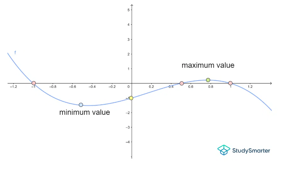
Graph for Example 7
The pink points represent the \(x\)-intercepts.
The yellow point represents the \(y\)-intercept.
In this case, we obtain two turning points for this graph:
- a minimum value between the roots \(x = –1\) and \(x=\frac{1}{2}\). This is indicated by the green point.
- a maximum value between the roots \(x=\frac{1}{2}\) and \(x = 1\). This is indicated by the blue point.
Cubic Function Graphs - Key takeaways
- A cubic graph has three roots and two turning points
- Sketching by the transformation of cubic graphs
| Form of Cubic Polynomial | Description | Change in Value |
y = ax3 | Varying a changes the cubic function in the y-direction | - If a is large (> 1), the graph becomes vertically stretched
- If a is small (0 < a < 1), the graph becomes flatter
- If a is negative, the graph becomes inverted
|
y = x3 + k | Varying k shifts the cubic function up or down the y-axis by k units | - If k is negative, the graph moves down k units
- If k is positive, the graph moves up k units
|
y = (x - h)3 | Varying h changes the cubic function along the x-axis by h units | - If h is negative, the graph shifts h units to the left
- If h is positive, the graph shifts h units to the right
|
- Graphing by factorisation of cubic polynomials
- Factorise the given cubic polynomial
- Identify the \(x\)-intercepts by setting \(y = 0\)
- Identify the \(y\)-intercept by setting \(x = 0\)
- Plot the points and sketch the curve
- Plotting by constructing a table of values
- Evaluate \(f(x)\) for a domain of \(x\) values and construct a table of values
- Locate the zeros of the function
- Identify the maximum and minimum points
- Plot the points and sketch the curve


