What is a differential equation?
When we have an equation that involves a series of derivatives, we call this a differential equation. When the derivatives are of a function of one variable, we call this an ordinary differential equation (ODE). When talking about a differential equation, we often talk about its order. Order means the highest derivative that is present in the equation. For example, the equation  is of order two, as the highest order derivative in the equation is second order.
When solving a differential equation, the aim is to find a function that satisfies the equation. This solution will not be unique, as with a derivative, a constant can be added to change the function but still satisfy the equation. The only way that the value of this constant can be found is by the addition of a boundary condition.
In a first order ordinary differential equation, we only need one boundary condition to satisfy the unknown. In general, for an order ordinary differential equation, we need n boundary conditions. A boundary condition specifies the value of the function at a certain point. This allows you to then work out the value of any unknown coefficients.
Verifying solutions of differential equations
When given a differential equation, if we get given a potential solution, we can verify whether it is valid or not. This involves working out all the derivatives used and then filling these in to see if the potential solution is suitable to satisfy the equation.
Verify that  is a solution to
  . (Note here that we use to represent
  , and to represent
  ).
).
Using the Product Rule, let us find the first and second derivative of y with respect to x.

Then
We can now fill in the values to get
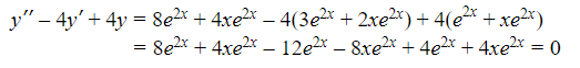
Hence the solution is verified.
Solving differential equations
At A level, we only need to know how to solve first order separable ordinary differential Equations. Separable refers to the fact that the two variables (normally x and y) can be separated and then split up to solve.
The form of a separable differential equation (for variables y and x, where y is a function of x) is  . We can then rearrange this to
 , and then integrate to get
 . Once integrated, this is our general solution for the differential equation. We can then apply any boundary conditions to find a specific solution if necessary.
It is worth noting that strictly speaking, we cannot manipulate in this way, as it is not a fraction but rather a Notation for the derivative. However, we can treat it like a fraction in this case.
Sketching a family of solution curves for differential equations
When we are finding a general solution for a differential equation, then we are left with constants in the general equation. These constants can be any value, and they would still satisfy the differential equation. The family of solution curves is the collection of the Functions with various values for the constants.
Find the general solution to  , and draw a graph showing this with four different particular solutions.

Below is a graph showing when C = -1, 0, 1, 2
 A family of solutions, with C = 2 green, C = 1 blue, C = 0 red and C = -1 purple, Tom Maloy - StudySmarter Originals


 .
. , so that means that the solution is of the form
  . This means we can fill in the two
  . Integrating the right-hand side, we get
  . On the left-hand side, this is a standard integral, given as
  .
. 
 . Note we have combined both the constants into one here. We can simplify this further to give
 .
. , with
 .
. .
.  , and the right-hand side integrates to
 .
. . This can simplify further to give
 .
.  , so we can fill this in to get
 .
. .
. . Water flows out of the tank at a rate proportional to the square root of the volume in the tank. Find
  .
.  , meaning
 .
.  , where a is a constant of proportionality.
 .
.  .
. , with solution
 .
.


